Mountain Pass

Many systems in physics or engineering can be modeled both by (partial) differential equations and an energy functional. Equilibrium states of such systems are then represented by solutions of the equations or by stationary points of the energy. For example, the potential energy is proportional to the elevation above the sea level. Hence it is small in valleys and large on mountains. The simplest critical points of the energy are at local minima (at the bottom of a valley) and at local maxima (at the top of a mountain). 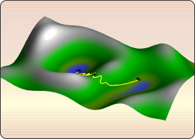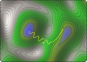But there are also other critical points - saddle points. Figures 1 and 2 show that if one wants to go from one valley to another one, one must cross a mountain range. In order to spend as little energy as possible, one chooses a path, that does not go any higher than it is absolutely necessary. Such a path must then go through a saddle point (a black star in the middle of the path on Figures 1 and 2) - a mountain pass point.

Fig. 1		Fig. 2

Even in more general applications, mountain pass points are critical points of the energy with the above described path property. In order to find them numerically, one can apply the Mountain Pass Algorithm [1]. The algorithm takes a path connecting two valleys and starts deforming it until an "optimal" path is reached - a path with the lowest maximal point among all possible paths. This point is a mountain pass.

	Fig. 3

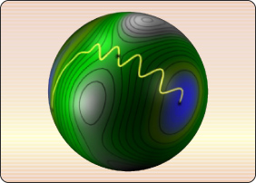
There are applications though where the energy is not defined on a linear space (like on a two dimensional plane in Figures 1 and 2) but on some more general surface (like a sphere in Figure 3 or even more general). The idea of the Mountain Pass Algorithm has been adapted even to such problems - it is called Constrained Mountain Pass Algorithm [2]. Here one has to deform the path on the given surface. It can be applied, e.g., to the Problem of the Fucik spectrum or the Traveling wave problem.