When solving PDEs with the finite volume method, one must choose a numerical flux function. We use a convex combination of the central flux $F^C$ and local Lax Friedrich flux $F^{LLF}$ to solve the Burgers equation.

\begin{align*}
&u_t + \left(\frac{u^2}{2}\right)_x =0\\
&\frac{du_j}{dt} =\frac{1}{\Delta x} \left[ \alpha_j \left(F_{j-1/2}^{LLF} -F_{j+1/2}^{LLF}\right) + (1-\alpha_j)\left(F_{j-1/2}^{C} – F_{j+1/2}^{C}\right) \right]
\end{align*}

The central flux is highly accurate but can lead to oscillating and thus unstable solutions. The local Lax Friedrich flux is stable but also dissipative. Therefore, we want to choose alpha so that the solution is stable and at the same time as accurate as possible. We train a Reinforcement Learning Agent to choose alpha. One agent performs locally in one grid cell. The action of agent j is $\alpha_j$ and the state is given by

\begin{equation*}
r_j=\frac{u_j – u_{j-1}}{u_{j+1} – u_{j}}.
\end{equation*}

The policy is a Neural Network with one hidden layer of size 10, a relu activation function in the first layer, and a hard sigmoid function in the output layer. The deep deterministic policy gradient (DDPG) approach is used to train the agent.

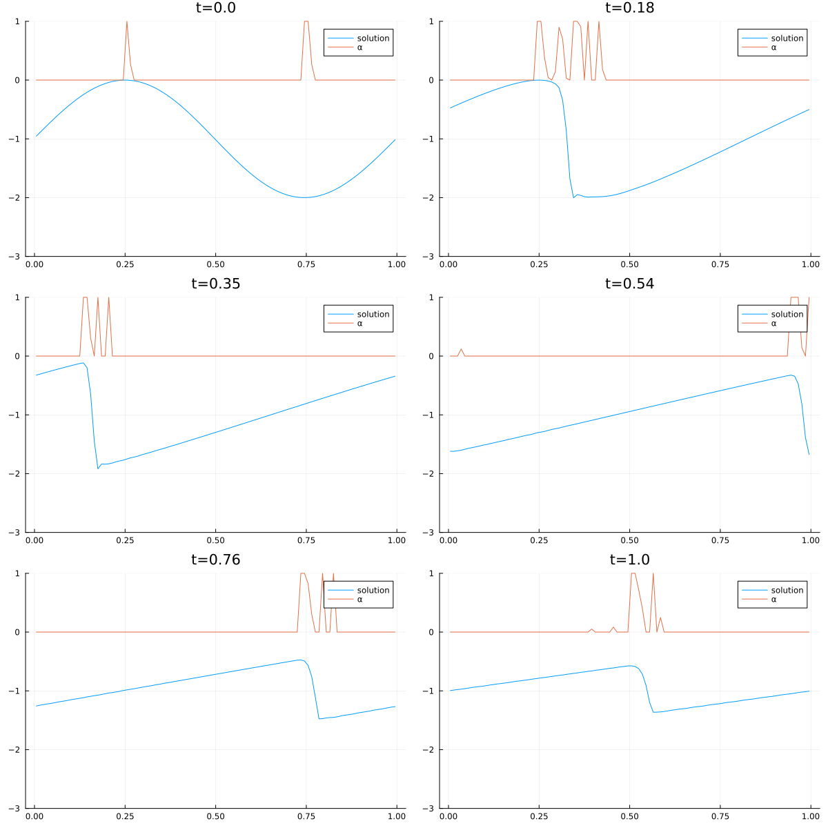
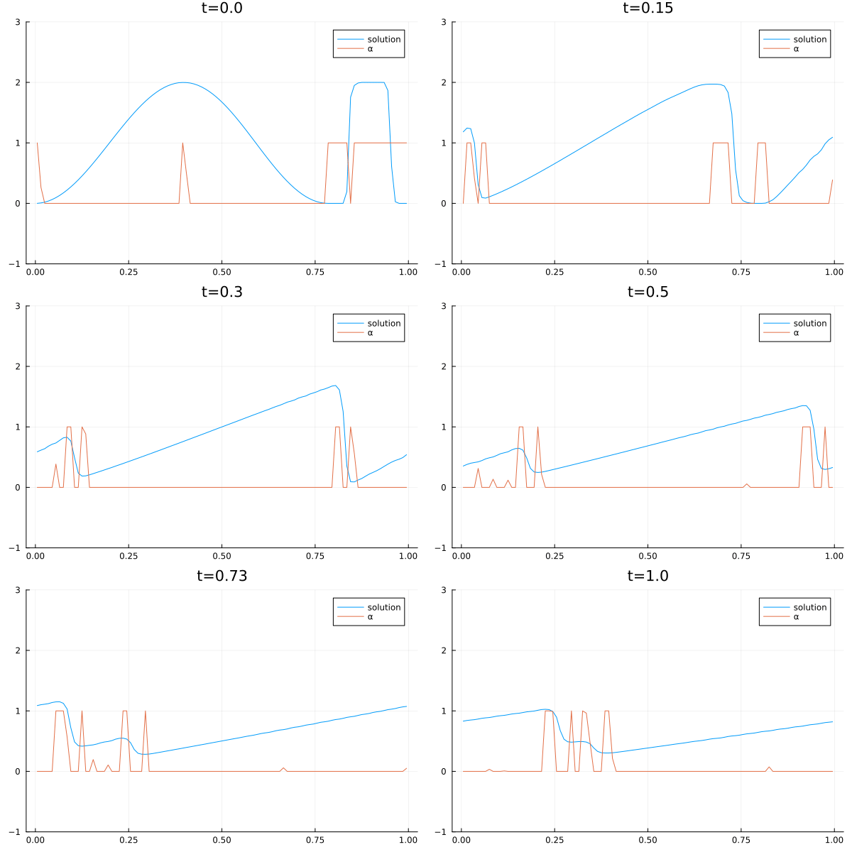
The video below shows the chosen amount of local Lax Friedrich flux and the resulting solution of the Burgers equation. The initial solution is a sine wave with two discontinuities. Randomly changed variants of this were used for training.

The agent performs well in unseen situations, e.g. negative sine wave, as shown below.