We solve the shallow water equations with DGSEM on a mesh with 103 elements and polynomial degree 12 in combination with subcell shock capturing and limiting, positivity preservation and handling of wet/dry regions.
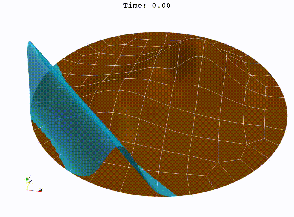
We solve the shallow water equations with DGSEM on a mesh with 103 elements and polynomial degree 12 in combination with subcell shock capturing and limiting, positivity preservation and handling of wet/dry regions.
In den neunziger Jahren wurden erstmals Ameisenalgorithmen von Marco Dorigo vorgestellt. Der erste Algorithmus war das sogenannte Ant System (AS), welches in der Bachelorarbeit implementiert wurde, um das Travelling Salesman Problem zu lösen. Dabei wird das Verhalten von Ameisen in einen Algorithmus übertragen, um den kürzesten Hamiltonkreis in einem Graphen zu finden. Die Ameisenalgorithmen bauen auf dem Prinzip auf, dass jede virtuelle Ameise, ausgehend von einem zufälligen Startknoten, einen Hamiltonkreis in dem gegebenen Graphen abläuft und auf dieser Tour dann Duftstoffe, sogenannte Pheromone, hinterlässt. Die hinterlassene Menge der Pheromone hängt dabei davon ab, wie lang die Tour einer Ameise ist. Durch die Duftstoffe werden andere Ameisen dazu angeregt, auch diesen Weg zu wählen. Je mehr Pheromone sich auf einer Kante befinden, desto wahrscheinlicher ist es, dass eine Ameise diese Kante in ihrer Tour wählt. Nach einigen Iterationen befindet sich also die größte Menge der Pheromone auf dem kürzesten Hamiltonkreis. Eine Erweiterung dieses Algorithmus ist das Ant Colony System (ACS), welches ebenfalls auf das Travelling Salesman Problem angewandt wurde. Einer der Unterschiede zum Ant System ist es, dass die Ameisen alle die gleiche Menge an Pheromonen auf ihrer Tour hinterlassen und außerdem die beste Ameise ausgewählt wird, welche eine zusätzliche Menge an Pheromonen auf ihrem Hamiltonkreis abgibt. Im Laufe der Jahre wurden weitere Modifikationen entwickelt, die sich auch auf andere Optimierungsprobleme anwenden lassen.
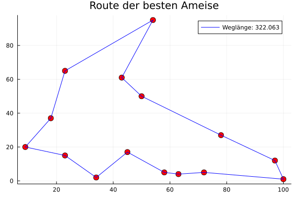
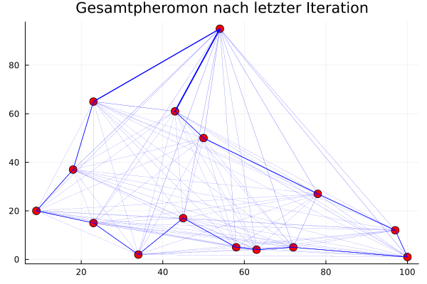
Abbildung: Beispiel für die Lösung des Travelling Salesman Problems mit dem ACS [1] M. Dorigo und T. Stuetzle, Ant Colony Optimization. MIT Press Ltd, 2004, isbn: 9780262042192
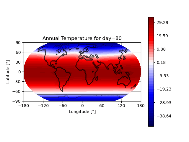
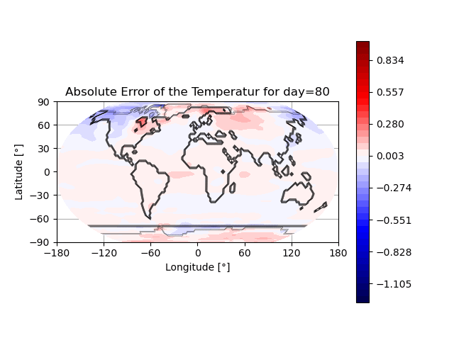
Recently, a lot of research has been done on the development of Neural Operators. The aim is to map infinite-dimensional functions to infinite-dimensional functions with neural networks. One approach is the Fourier Neural Operator [1]. We use this model to estimate the annual temperature based on the global land-sea-ice distribution. The input of the neural network is the earth’s geography, the output is the global temperature over one year. The training and testing data set is generated with the simulation framework “Klimakoffer” (for more information see Snapshot: Numerical simulations of earth’s climate and [2]).
The best results are achieved when using 4 Fourier integral operator layers, 16 Fourier modes, and a network width of 20. The model thus has 52 433 557 trainable parameters. The remaining specifications are as chosen by Li et al. [1]. It took 4 hours and 26 minutes to train the model on an NVIDIA GeForce RTX 3090 GPU and 0.77 seconds to evaluate it for one given example on a CPU. A relative L2 loss of approximately 0.0025 was achieved during training.
The first video shows one exemplary output. The second animation visualizes the difference between the temperature calculated by the FNO model and the “true” temperature determined by the framework “Klimakoffer”.
References:
[1] Li, Z., Kovachki, N., Azizzadenesheli, K., Liu, B., Bhattacharya, K., Stuart, A., Anandkumar, A. (2020). “Fourier Neural Operator for Parametric Partial Differential Equations”, arXiv, https://arxiv.org/abs/2010.08895
[2] Zhuang, K., North, G.R., Stevens, Mark J. (2017). “A NetCDF version of the two-dimensional energy balance model based on the full multigrid algorithm”, SoftwareX
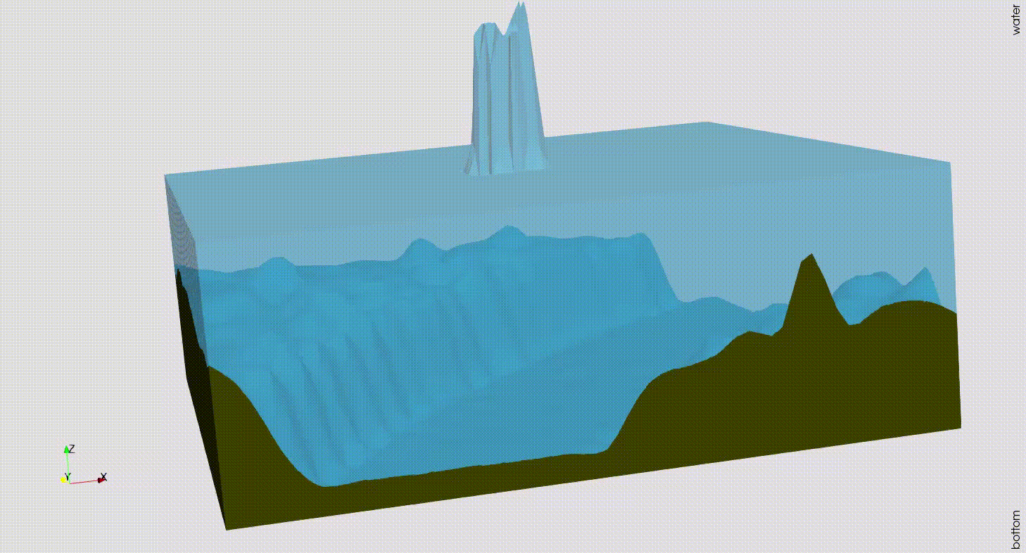
Back in the summer of 2021, severe floods struck Western Germany, resulting in several cities and villages being destroyed and hundreds of people losing their lives. Modelling and predicting those floods can be crucial for investigating such natural disasters. The shallow water equations are a system of physical conservation equations that can model water flow over a given domain. The two dimensional shallow water equations are given as follows:
\begin{equation*}
\left\{\begin{aligned}
\frac{\partial}{\partial t} h + \left( h v_1\right)_x + \left( h v_2\right)_y =0&\\
\frac{\partial}{\partial t} hv_1 + \left( hv_1^2 + \frac{1}{2} gh^2\right)_x + \left(h v_1v_2\right)_y &= -ghb_x\\
\frac{\partial}{\partial t}h v_2 + \left( hv_1v_2\right)_x + \left(hv_2^2 +\frac{1}{2} gh^2\right)_y &= -ghb_y
\end{aligned}\right.
\end{equation*}
Here the variable $b$ describes the underlying bottom topography function of the domain. As this system is set up of hyperbolic partial differential equations, we use the numerical solver Trixi.jl to approximate the solutions. This solver is part of the trixi-framework. Trixi.jl already implemented the shallow water equations but did not yet offer the functionality to include real-world topography data into the calculations. Therefore the add-on TrixiBottomTopography.jl has been included in the trixi-framework. This tool uses B-spline interpolation approaches to remodel the bottom topography function from real-world data, which is often given as elevation data at specific points. One example is the DGM1 data set which provides uniformly spaced elevation data of the whole German state of North Rhine-Westphalia. Using this data set and the functionalities implemented in Trixi.jl as well as TrixiBottomTopography.jl, we can simulate a dam break problem over a section of the Rhine river valley.
In this talk, we present the class of split form discontinuous Galerkin methods. The notion of split form refers to different interpretations of the non-linear terms in the fluid dynamics equations. For instance the advective part of the momentum flux can be cast in analytically equivalent forms such as the advective form, or the conservative form, or convex combinations of both forms. While these forms are analytically equivalent for smooth solutions, it is interesting to understand that their discrete forms might have strongly different properties. It turns out that specific underlying split forms of the fluid equations give discontinuous Galerkin (DG) approximations with special favourable properties such as, kinetic energy preservation, energy consistency, pressure equilibrium preservation and even entropy conservation/stability. The most important improvement that can be observed is drastically increased non-linear robustness of the DG discretization, in particular when simulating under-resolved turbulence. A necessary ingredient to retain fully discrete conservation when using split formulations is the so-called summation-by-parts (SBP) property of the discrete derivative and integral operator. It turns out hat specific DG discretizations, such as the Legendre-Gauss-Lobatto (LGL) spectral element method, satisfy the SBP property. We will further discuss in this talk that it is possible to construct compatible low-order finite volume discretizations on the LGL subcell grid, such that a convex blending of the high-order DG method with the robust low-order method is feasible. This allows to construct provably positive hybrid discretizations that enable simulations of problems with strong shock waves, such as e.g. an astrophysical jet with Ma=2000.
Link to the Talk: https://cassyni.com/events/VrFL7HmR9YjHyFJvFcZNjP
We solve the compressible Euler equations of gas dynamics with a fourth-order accurate entropy-stable discontinuous Galerkin (DG) method and combine it with a first-order accurate finite volume (FV) method at the node level to impose positivity of density and pressure [1,2].
The initial condition of this problem is given by:
\[
\begin{array}{rlrl}
\rho (t=0) &= \frac{1}{2}
+ \frac{3}{4} B,
&
p (t=0) &= 0.1, \\
v_1 (t=0) &= \frac{1}{2} \left( B-1 \right),
&
v_2 (t=0) &= \frac{1}{10} \sin(2 \pi x),
\end{array}
\]
with $B=\tanh \left( 15 y + 7.5 \right) – \tanh(15y-7.5)$, where $\rho$ is the density, $\vec{v}=(v_1,v_2)$ is the velocity, and $p$ is the pressure.
The video shows the evolution of the density in time using $1024^2$ and degrees of freedom. We use the entropy-conservative and kinetic energy preserving flux of Ranocha [3] for the volume fluxes and the Rusanov solver for the surface fluxes of the DG and FV methods. During this simulation, the FV method acts on average in 0.000086% of the computational domain, and never more than 0.002% of the computational domain at a specific time.
References
[1] A. M. Rueda-Ramírez, G. J. Gassner, A Subcell Finite Volume Positivity-Preserving Limiter for DGSEM Discretizations of the Euler Equations, WCCM-ECCOMAS2020, pp. 1–12.
[2] A. M. Rueda-Ramírez, W. Pazner, G. J. Gassner, Subcell limiting strategies for discontinuous galerkin spectral element methods, Computers & Fluids 247 (2022) 105627.
[3] H. Ranocha, Generalised summation-by-parts operators and entropy stability of numerical methods for hyperbolic balance laws, Cuvillier Verlag, 2018.