The shallow water equations are a well-known and often used physical model to simulate shallow water flow within given domains such as oceans. They are a system of hyperbolic partial differential equations and consist of conservation equations.

The numerical solver Trixi.jl is used to find approximate solutions to the equations. The shallow water equations are already embedded in this framework, but Trixi.jl does not yet allow for the appearance of dry sub-regions. Some strategies are combined and implemented to resolve the wet-dry problem resulting in a stable and well-balanced scheme: We use the positivity-preserving limiter by Zhang and Shu [1], the hydrostatic reconstruction method by Chen and Noelle [2] and a strategy to identify and mark dry cells.

A standard test exists to check for accuracy, namely the parabolic bowl test by Niklas Wintermeyer [3], first presented by William Thacker [4]. We use a StructuredMesh with 75625 elements and polynomial degree five. Since it has periodic analytical solutions, we can show the precision by realizing the initial state and its linear structure are recovered after one period. In the left picture, the whole domain is shown. In the right image, a slice at $y=0$ is visualized. Both are snapshots after one period:

We also use the TrixiBottomTopography.jl package by Maximilian Bertrand to account for real-world bottom topography data from the DGM1 data set. We give the simulation of flooding on the Rhine River valley using a TreeMesh with 1024 elements polynomial degree six and outflow boundary conditions:

References:
[1] Zhang, X. and Chi-Wang, S. (2011). Maximum-principle-satisfying and positivity-preserving high-order schemes for conservation laws: survey and new developments. Proc. R. Soc. A. 467:2752–2776. http://doi.org/10.1098/rspa.2011.0153
[2] Chen, G. and Noelle, S. (2017). A New Hydrostatic Reconstruction Scheme Based on Subcell Reconstructions. SIAM Journal on Numerical Analysis, 55, 758-784. https://doi.org/10.1137/15M1053074
[3] Wintermeyer, N.(2018). A novel entropy stable discontinuous Galerkin spectral element method for the shallow water equations on GPUs. Dissertation, Universität zu Köln. https://kups.ub.uni-koeln.de/9234/
[4] Thacker, W. (1981). Some exact solutions to the nonlinear shallow-water wave equations. Journal of Fluid Mechanics, 107, 499-508. doi:10.1017/S0022112081001882

Back in the summer of 2021, severe floods struck Western Germany, resulting in several cities and villages being destroyed and hundreds of people losing their lives. Modelling and predicting those floods can be crucial for investigating such natural disasters. The shallow water equations are a system of physical conservation equations that can model water flow over a given domain. The two dimensional shallow water equations are given as follows:

\begin{equation*}
\left\{\begin{aligned}
\frac{\partial}{\partial t} h + \left( h v_1\right)_x + \left( h v_2\right)_y =0&\\
\frac{\partial}{\partial t} hv_1 + \left( hv_1^2 + \frac{1}{2} gh^2\right)_x + \left(h v_1v_2\right)_y &= -ghb_x\\
\frac{\partial}{\partial t}h v_2 + \left( hv_1v_2\right)_x + \left(hv_2^2 +\frac{1}{2} gh^2\right)_y &= -ghb_y
\end{aligned}\right.
\end{equation*}

Here the variable $b$ describes the underlying bottom topography function of the domain. As this system is set up of hyperbolic partial differential equations, we use the numerical solver Trixi.jl to approximate the solutions. This solver is part of the trixi-framework. Trixi.jl already implemented the shallow water equations but did not yet offer the functionality to include real-world topography data into the calculations. Therefore the add-on TrixiBottomTopography.jl has been included in the trixi-framework. This tool uses B-spline interpolation approaches to remodel the bottom topography function from real-world data, which is often given as elevation data at specific points. One example is the DGM1 data set which provides uniformly spaced elevation data of the whole German state of North Rhine-Westphalia. Using this data set and the functionalities implemented in Trixi.jl as well as TrixiBottomTopography.jl, we can simulate a dam break problem over a section of the Rhine river valley.

Autonomous vehicles will be an integral part of our environment and will have a significant impact on transportation and other industries. In this context, drones, so-called UAVs will be used for aerial transportation. Due to the high information density, motion planning is a fundamental problem in the autonomous movement of vehicles.
In the future, drones should transport goods or perhaps people in a fast, safe and thus collision-free manner. In doing so, the drone should be able to perform all calculations quickly, accurately and autonomously. Therefore, it makes sense to develop algorithms that meet these requirements.
As part of a bachelor thesis, a method [1] was investigated that uses uniform B-splines to replan a drone’s trajectory in the presence of a potential collision. This method formulates the task of replanning the trajectory as the solution to a non-linear optimization problem.
\begin{align*}
E=\lambda_{ep}(p(t_{ep})-p_{ep})^{2}+\lambda_{ep}(p'(t_{ep})-p’_{ep})^{2} + \lambda_{c} \int_{t_{min}}^{t_{max}}c(p(t))||p'(t)||dt + \sum_{i=2}^{4}\int_{t_{min}}^{t_{max}}\lambda_{q}(p^{(i)}(t))^{2}dt
\end{align*}
With this simplified equation, three cost terms are considered: Endpoint error, collision cost and quadratic derivative cost. With the goal of computing an efficient and collision-free trajectory, an iterative process is used to construct a B-spline curve such that it follows a pre-planned and optimal trajectory. The focus of the analysis was on the selection of the control parameters λep, λc, λq, as well as the number of control points to be optimized and the resulting properties of the optimized trajectory. Using a uniform knot vector, the B-spline is expanded to include control points whose spatial coordinates are determined using nonlinear optimization so that the objective function is minimized. Due to the properties of B-splines, upcoming segments can be locally optimized so that a collision is prevented. The use of a uniform knot vector allows an efficient replanning of the trajectory in real time, which can be performed autonomously by a drone. The following figure shows one result.

[1] Vladyslav Usenko, Lukas von Stumberg, Andrej Pangercic, Daniel Cremers, Real-Time Trajectory Replanning for MAVs using Uniform B-splines and a 3D Circular Buffer, Technical University of Munich, 2017, https://arxiv.org/abs/1703.01416.

In a previous snapshot, the two-dimensional energy balance model has been already presented:\begin{align*}
C(\hat{r})\frac{\partial T(\hat{r},t)}{\partial t} +A+BT(\hat{r},t)= \nabla\cdot(D(\hat{r})\nabla T(\hat{r},t)) + QS(\hat{r},t)(1-a(\hat{r}))
\end{align*}
The model is based on the assumption of a static surface distribution of the surface types land, ocean, sea ice and snow. However, climate change at an increasing rate is also affecting surface types seasonally as well as permanently over the years. Melting ice and snow masses worldwide are a consequence of this, affecting not only snow and sea ice distribution, but also that of oceans and land surfaces through rising sea ice levels.
Therefore, for more accurate climate modeling with this EBM, it is interesting to modify the model with respect to a time-dependent surface distribution. This modification directly affects the model parameters albedo, solar forcing, and heat capacity, requiring the following reformulation of the model:
\begin{align*}
C(\hat{r},t)\frac{\partial T(\hat{r},t)}{\partial t} +A+BT(\hat{r},t)= \nabla\cdot(D(\hat{r})\nabla T(\hat{r},t)) + QS(\hat{r},t)(1-a(\hat{r},t))
\end{align*}
As part of a bachelor’s thesis, two options were presented for introducing a seasonal sea ice distribution into the EBM by using and modifying simulations from the ‘Klimakoffer‘. Similar approaches are also conceivable for the other surface types.
One possibility is to process documented measurements of sea ice distribution, available for example from institutions such as the NSIDC (National Snow and Sea Ice Data Center) or NASA, so that a monthly change in sea ice distribution at the edge of the sea ice extent at the two poles can be mapped using a specially developed algorithm.

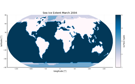
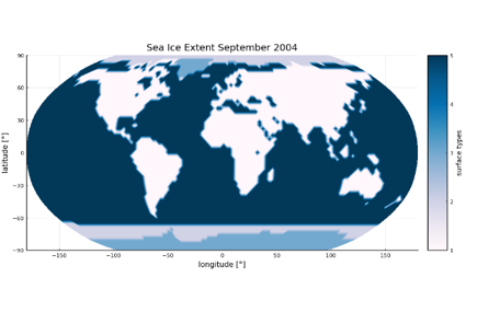
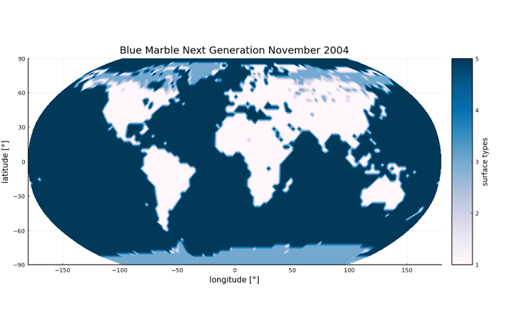
A second option is to directly read in satellite images and categorize the color values of the image’s pixels and map them to the surface types required in the EBM. Here, as an example, a satellite image of the Blue Marble series from 2004 of NASA was read in and categorized on the basis of the color values to the different surface types.

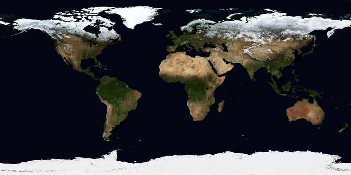
Image from NASA’s Blue Marble Next Generation [3]

[1] North, G.R.; Mengel, J.G.; Short, D.A. (1983). Simple Energy Balance Model Resolving the Seasons and the Continents’ Application to the Astronomical Theory of the Ice Ages. Journal of Geophysical Research.
[2] Zhuang, K.; North, G.R.; Stevens, Mark J. (2017). A NetCDF version of the two-dimensional energy balance model based on the full multigrid algorithm. SoftwareX.
[3] EOS Project Science Office at NASA Goddard Space Flight Center, Blue Marble Next Generation, 2004, https://visibleearth.nasa.gov/collection/1484/blue-marble.