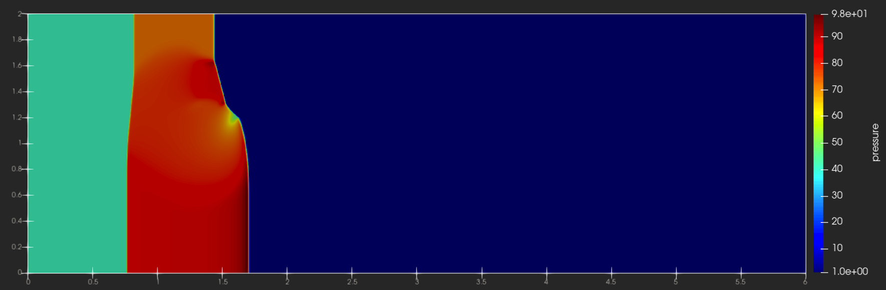
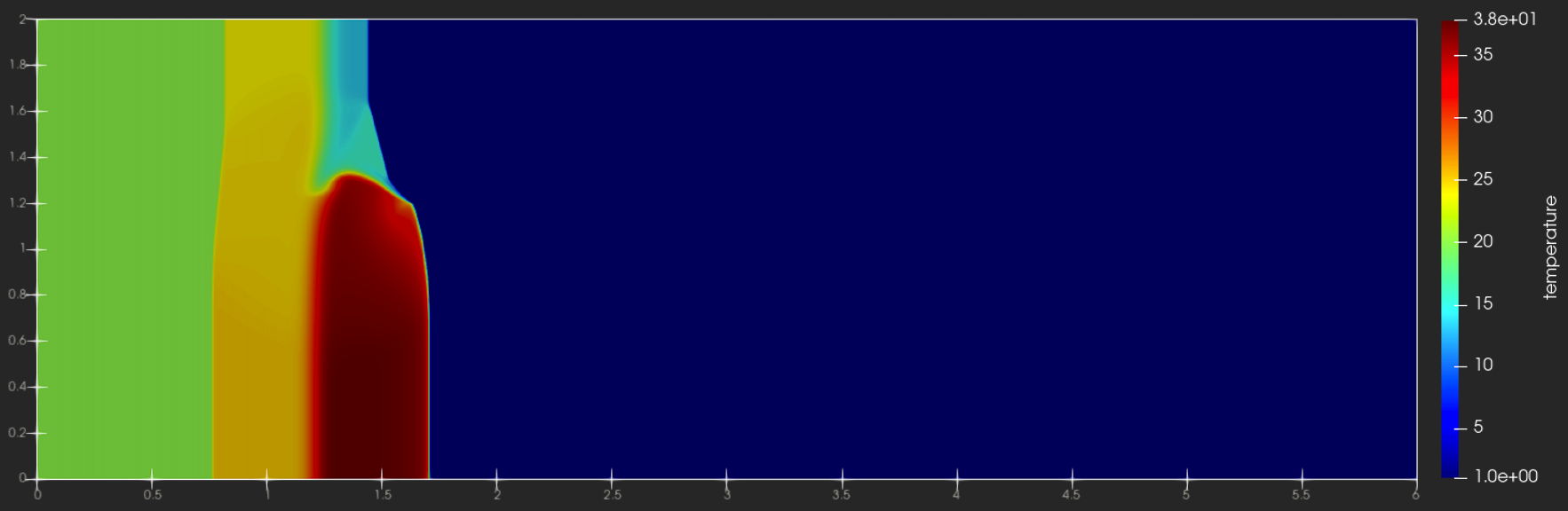
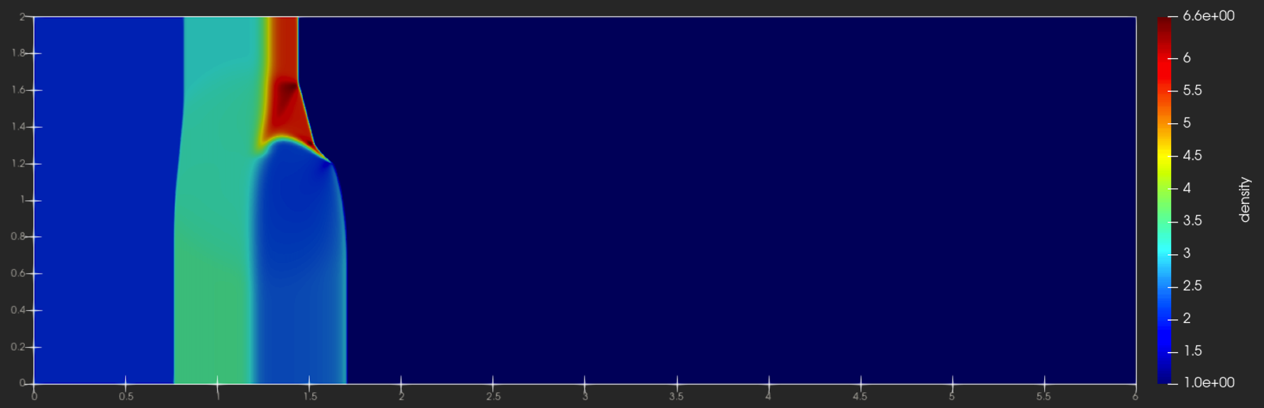
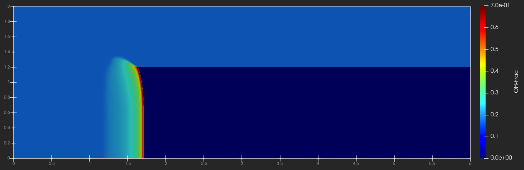
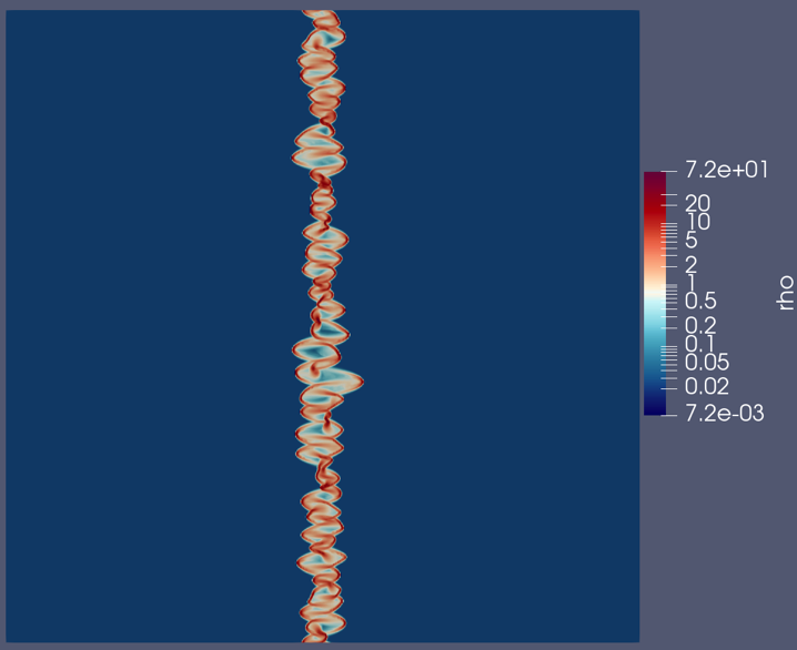
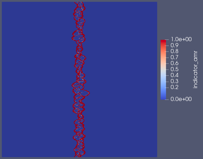
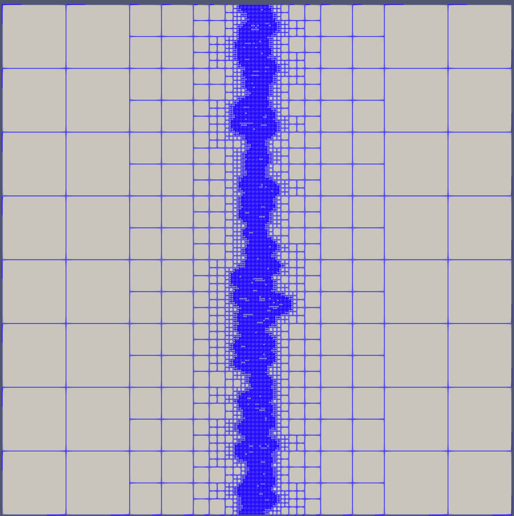
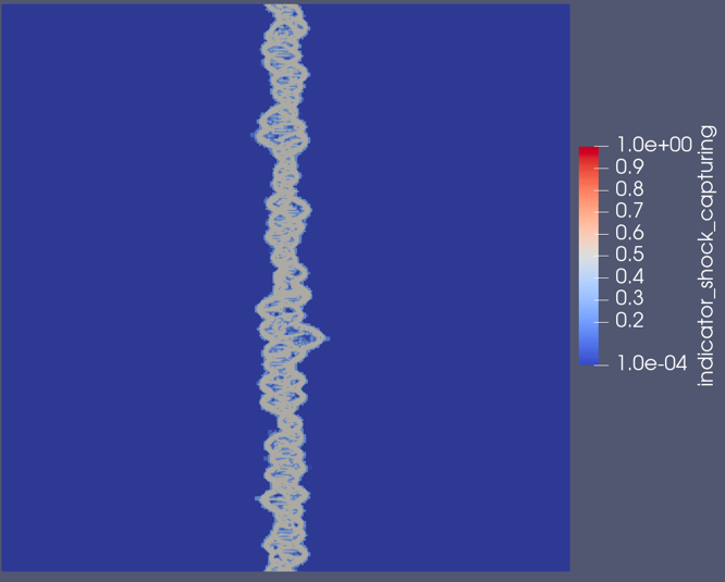
Simulation of the viscous flow past a cylinder with a discontinuous Galerkin spectral element method on a hierarchical Cartesian mesh with adaptive mesh refinement (AMR). The polynomial degree is N = 3 and the mesh uses five refinement levels. The cylinder boundary is imposed with an immersed boundary method (IBM) based on volume penalization [1], which adds a source term to the compressible Navier-Stokes equations,
$$
\partial_t \mathbf{u} + \nabla \cdot \vec{\mathbf{f}} (\mathbf{u},\nabla \mathbf{u}) = \underbrace{\beta (\mathbf{u}_s – \mathbf{u})}_{\text{IBM source}},
$$
where $\mathbf{u}$ is the vector of conservative quantities, $\vec{\mathbf{f}}$ is the Navier-Stokes flux, $\beta$ is the penalty parameter, and $\mathbf{u}_s$ is an imposed state. For this simulation, $\mathbf{u}_s$ mimics an isothermal no-slip wall boundary condition.

The simulation was obtained with the open-source code FLUXO (https://github.com/project-fluxo/fluxo).

References
[1] Kou, J., Joshi, S., Hurtado-de-Mendoza, A., Puri, K., Hirsch, C., & Ferrer, E. (2022). Immersed boundary method for high-order flux reconstruction based on volume penalization. Journal of Computational Physics, 448, 110721.

Simulation of an asymmetric two-dimensional stiff multi-species reacting flow for the compressible Euler equations. The computation domain [0,6]x[0,2] of this detonation problem is split into three zones. Zone A [0,0.5]x[0,2] as well as zone B (0.5,6]x[1.2,2] is filled with burnt gas, namely O2,OH and H2O. The last zone C (0.5,6]x[0,1.2) contains unburnt gas, namely H2 and O2.

The reacting model consists of two reactions H2+O2->2OH, 2OH+H2->2H2O and five species H2,O2,OH,H2O,N2 whereas reaction 1 has a smaller ignition temperature as well as a much faster chemical rate than reaction 2. Species N2 acts as a dilute catalyst here.

This example has been calculated using Trixi.jl with a P4est mesh using 3072x1024=3.145.728 elements, Dirichlet boundary conditions in x-direction as well as solid wall boundaries in y-direction. The final time is T = 0.1. The convection part is solved with FV whereas the chemical network is solved with KROME. (Note: Not all of these features are currently available in the main code of Trixi.jl.)

Pressure distribution at final time T=0.1:

Temperature distribution at final time T=0.1:

Density distribution at final time T=0.1:

OH-fraction distribution at final time T=0.1:

Earth’s climate is changing due to human activity. Therefore, the ability to predict future climate change is of utmost importance if we want to reduce the human interference with the climate system (climate change mitigation) and our vulnerability to the harmful effects of climate change (climate change adaptation).

It is possible to model the time-dependent local temperatures on the globe using a simple two-dimensional energy balance model [1,2],
$$ C(\vec{x}) \frac{\partial T}{\partial t} + A + BT = \nabla \cdot \left( D(\vec{x}) \nabla T \right) + Q S(\vec{x},t) (1-a(\vec{x})), $$
where $T$ is the local temperature; $C(\vec{x})$ is the local heat capacity for a column of air on land, water or ice; the term $A+BT$ models the outgoing long-wave radiation, where $A$ depends on the amount of green-house gases in the atmosphere and $B$ models several feedback effects; $D$ is a latitude-dependent diffusion coefficient; and the last term includes the heat input in the system, where $Q$ is the solar radiation at earth’s position in the solar system, $S$ is the seasonal and latitudinal distribution of insolation, which depends on orbital parameters, such as the eccentricity of earth’s orbit, and the precession and tilt of earth’s rotation axis, and $a(\vec{x})$ is the local albedo, which measures the reflection of solar radiation and depends on the surface cover.

We developed a julia code that implements the EBM model on the sphere surface and used it to describe the mean temperatures on the globe assuming a constant atmospheric CO$_2$ concentration (of year 1950). The results are presented in the animation.

[1] North, G.R.; Mengel, J.G.; Short, D.A. (1983). Simple Energy Balance Model Resolving the Seasons and the Continents’ Application to the Astronomical Theory of the Ice Ages. Journal of Geophysical Research.
[2] Zhuang, K.; North, G.R.; Stevens, Mark J. (2017). A NetCDF version of the two-dimensional energy balance model based on the full multigrid algorithm. SoftwareX.

Io is the most volcanically active body of the solar system. Furthermore, it is embedded in Jupiter’s magnetic field, the largest and most powerful planetary magnetosphere of the solar system. Due to its strong volcanic activity, Io expels ions and neutrals, which are in turn ionized by ultraviolet and electron impact ionization, forming a plasma torus around Jupiter [1,2]. As Io moves inside the plasma torus, elastic collisions of ions and neutrals inside its atmosphere generate a magnetospheric disturbance that propagates away from Io along the background magnetic field lines at the Alfvén wave speed. This phenomenon creates a pair of Alfvén current tubes that are commonly called Alfvén wings, which have been observed by several flybys [1].

The figure shows the momentum (non-dimensional) and magnetic field of the plasma that surrounds Io, obtained with the magneto-hydrodynamic (MHD) plasma model of FLUXO*. The Alfvén wings can be observed as disturbances of both the background magnetic and momentum fields. In yellow is the trajectory of the I31 flyby of the Galileo spacecraft, which visited Io in 2001 [1]. The Galileo spacecraft is also depicted (not to scale). A 3D model of the moon’s surface developed by NASA [3] was superposed on the simulation results.

*FLUXO (www.github.com/project-fluxo/fluxo) is an MPI parallel high-order Discontinuous Galerkin code, which supports unstructured curvilinear hexahedral grids, and is able to perform Adaptive Mesh Refinement (AMR).

[1] M. Kivelson, K. Khurana, C. Russell, R. Walker, S. Joy, J. Mafi, GALILEO ORBITER AT JUPITER CALIBRATED MAG HIGH RES V1.0, GO-J-MAG-3-RDR-HIGHRES-V1.0, Technical Report, NASA Planetary Data System, 1997.
[2] J. Saur, F. M. Neubauer, J. E. P. Connerney, Plasma interaction of Io with its plasma torus, 2004.
[3] https://solarsystem.nasa.gov/resources/2379/io-3d-model/

[1] Machida, Mami, Mitsuru R. Hayashi, and R. Matsumoto.
“Global simulations of differentially rotating magnetized disks:
Formation of low-beta filaments and structured coronae.”
The Astrophysical Journal Letters 532.1 (2000): L67.
[2] Markert et al. “A Discontinuous Galerkin Method with Sub‑Cell Adaptive Shock Capturing for
FLASH” (in preparation)
[3] http://flash.uchicago.edu/

Here we are simulating a gingerbread man, whereby the gingerbread man itself has 861 unstructured quadrilateral elements. For the run parameters, we used polydeg = 10 with the compressible Euler equations and the manufactured (convergence test) solution. The visualization is done on nvisnodes=12 uniform points in each direction, on each element.

We thank Prof. Dr. Andrew Winters (https://liu.se/en/employee/andwi94) for providing this video/simulation.

We present in-viscid and viscous simulations of a Kelvin-Helmholtz instability using second a order accurate monotoniced-central finite volume (FV) method and a fourth order accurate discontinuous Galerkin (DG) method. The initial condition is given by [1]:

$$\rho (t=0) = \frac{1}{2}
+ \frac{3}{4} B,
~~~~~~~~~
p (t=0) = 1,~~~~~~~~~~
$$

$$
v_1 (t=0) = \frac{1}{2} \left( B-1 \right),
~~~~~~~
v_2 (t=0) = \frac{1}{10} \sin(2 \pi x),
$$

with $$B=\tanh \left( 15 y + 7.5 \right) – \tanh(15y-7.5).$$

We first present the FV results at end time $t=3.7$, which are computed using a monotoniced-central second order discretization of the Euler equations of gas dynamics on uniform grids.

The next results use a fourth order DG discretization of the Navier-Stokes equations on uniform grids using $Re=320.000$ at end time $t=3.7$. The highest resolution (4096² DOFs) is a direct numerical simulation (DNS) of the problem, where all scales are resolved.

It is remarkable that the numerical dissipation of the second order FV scheme causes the in-viscid simulation with 2048² DOFs to look very similar to the viscous DNS solution at $Re=320.000$.

[1] A.M. Rueda-Ramírez, G.J Gassner (2021). A Subcell Finite Volume Positivity-Preserving Limiter for DGSEM Discretizations of the Euler Equations. https://arxiv.org/pdf/2102.06017.pdf

We are interested in the accuracy of the finite volume scheme, on a LGL subcell grid induced by a LGL-DGSEM discretization. For comparison, we look at a Kelvin-Helmholtz-Instability test problem, simulated with 4² LGL nodes per element and 32² elements, i.e. 128² spatial degrees of freedom. The high-order DGSEM uses the entropy-conserving split-form powered by the flux of Chandrashekar in the volume, and the HLLC flux at the element interfaces. Positivity is controlled by adding subcell FV where the positivity is not fulfilled with the amount needed. All FV discretizations use the HLLC flux at the element interfaces and at the subcell interfaces as well.  

The first results show the high-order DGSEM result, which is formally 4^th order accurate for smooth problems:

The next result uses a subcell finite volume approximation on the LGL-subcell grid, directly, i.e. without spatial reconstruction (piecewise constant approximation). The result is very dissipative:

The last results show the improvement when using a piecewise linear reconstruction with monotonized-central slope limiter on the LGL-subcell grid. The reconstruction is inner-element only, as it does not use element neighbor information. Thus, at the very first and very last LGL subcell, no reconstruction is used. Still, the accuracy is recovered nicely by this simple modification of the subcell FV scheme: