DGSEM simulations of the two-dimensional Euler equations considering the astrophysical jet with Mach number $\textrm{Ma} \approx 2000$ [1].
The computational domain, $\Omega = [-0.5,0.5]^2$, is filled with a mono-atomic gas ($\gamma = 5/3$) at rest with
\begin{equation}
\rho(x,y) = 0.5, \qquad
p(x,y) = 0.4127, \qquad
v_1(x,y) = 0, \qquad
v_2(x,y) = 0,
\end{equation}
and on the left boundary there is a hypersonic inflow with
\begin{equation}
\rho(-0.5,y_B) = 5, ~
p(-0.5,y_B) = 0.4127, ~
v_1(-0.5,y_B) = 800, ~
v_2(-0.5,y_B) = 0,
\end{equation}
for $y_B \in [-0.05, 0.05]$, which corresponds to a Mach number of $\textrm{Ma}=2156.91$ with respect to the speed of sound of the jet gas, and $\textrm{Ma}=682.08$ with respect to the speed of sound of the ambient gas.
A spatial resolution of $256\times 256$ quadrilateral elements, a polynomial degree of $N=3$, and four different CFL numbers are used.
The simulations are stabilized by using two different subcell limiting approaches, the monolithic convex limiting (MCL) and the FCT/IDP limiting.
The resulting density contours at $t=10^{-3}$:
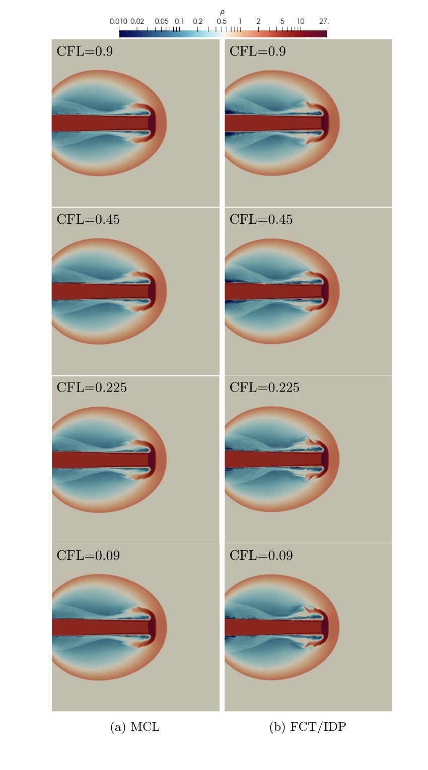
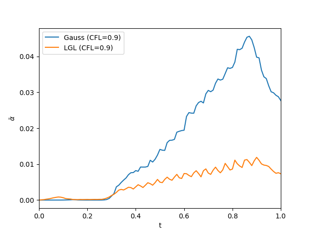
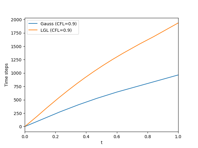
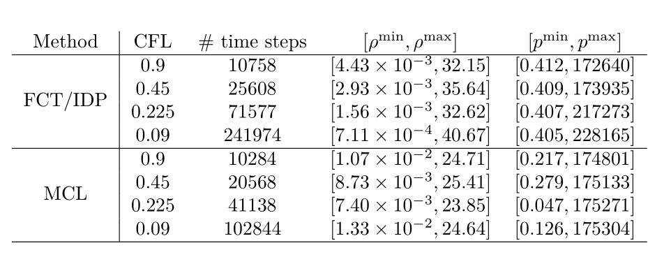
The dependence of the spatial discretization on the time-step size for FCT/IDP methods causes the number of vortical structures to be highly dependent on the CFL number and the total number of time steps to be not inversely proportional to the CFL number.
In fact, the amount of dissipation is reduced for small CFL numbers, which leads to lower minimum densities and higher maximum pressures in FCT/IDP, as can be seen in this Table.
References
[1] Rueda-Ramírez, A., Bolm, B., Kuzmin, D. & Gassner, G. (2023). Monolithic Convex Limiting for Legendre-Gauss-Lobatto Discontinuous Galerkin Spectral Element Methods. arXiv preprint arXiv:2303.00374