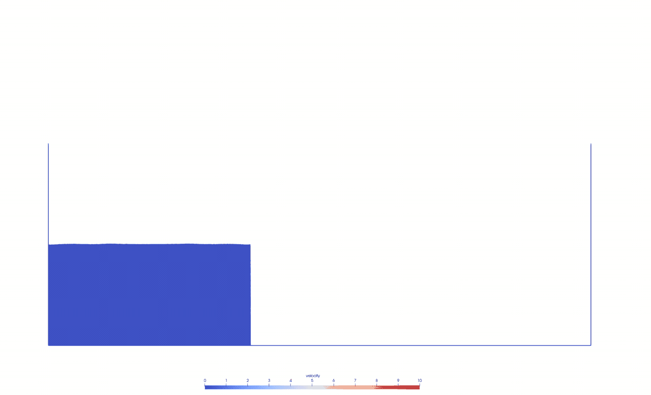
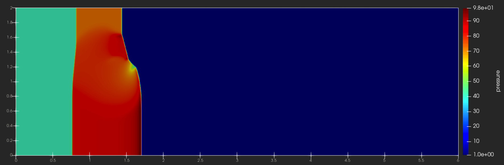
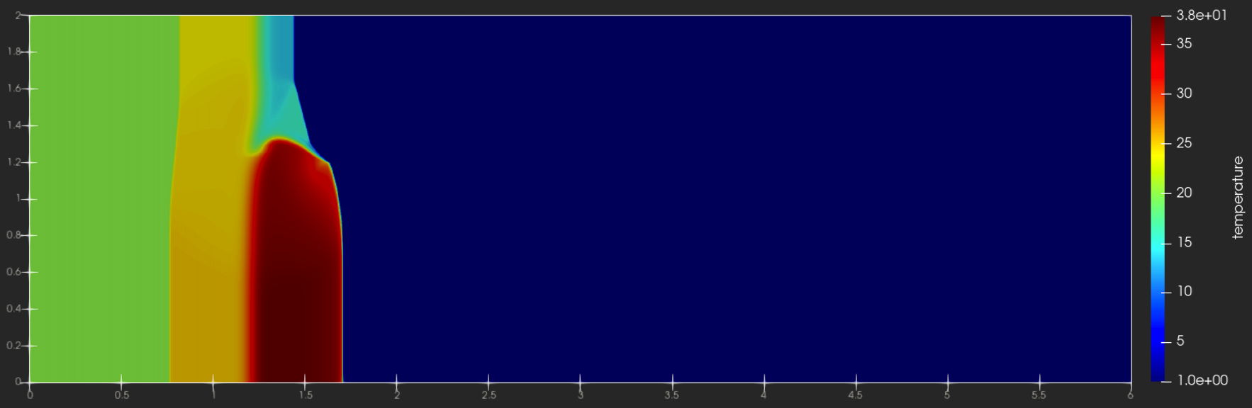
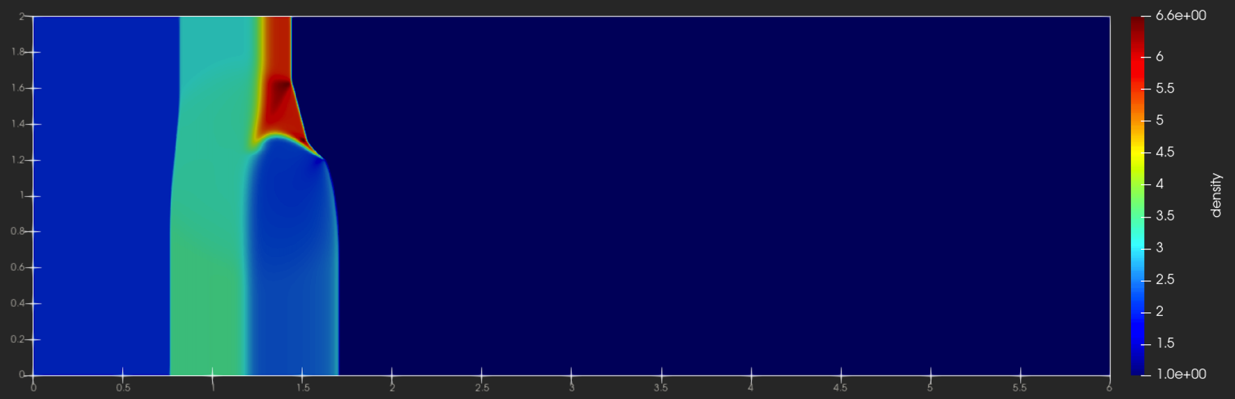
We solve the multi-component magneto-hydrodynamics (MHD) equations using a hybrid finite volume (FV)/discontinuous Galerkin (DG) method [1], which combines the two discretization approaches at the node level. To test the robustness of the hybrid FV/DG method, we compute a modification of the Orszag-Tang vortex problem [2], where we use two ion species and initialize the flow with a sharp interface at $y=0$:
\[
\begin{array}{rlrl}
\rho^1(x,y,t=0) &= \begin{cases}
{25}/{36 \pi} & y \ge 0 \\
10^{-8} & y < 0
\end{cases} ,
&\rho^2(x,y,t=0) &= \begin{cases}
10^{-8} & y < 0\\
{25}/{36 \pi} & y \ge 0
\end{cases} , \\
v_1 (x,y,t=0) &= – \sin (2 \pi y),
&v_2 (x,y,t=0) &= \sin (2 \pi x), \\
B_1 (x,y,t=0) &= -\frac{1}{\sqrt{4 \pi}} \sin (2 \pi y),
&B_2 (x,y,t=0) &= -\frac{1}{\sqrt{4 \pi}} \sin (4 \pi x). \\
p (x,y,t=0) &= \frac{5}{12 \pi},
& & \\
\end{array}
\]
where $\rho^1$ is the density of the first ion species, $\rho^2$ is the density of the second ion species,$\vec{v}=(v_1,v_2)$ is the plasma velocity, $\vec{B}=(B_1,B_2)$ is the magnetic field, and $p$ is the plasma pressure (without magnetic pressure).
The fourth-order DG method delivers high accuracy, but fails to describe shocks and material interfaces. Therefore, we use a modal indicator [3] to detect the elements where the solution changes abruptly. In those elements, we combine the DG method with a robust lower order FV scheme locally (at the node level) to impose TVD-like conditions on the density of the ion species,
\[
\min_{k \in \mathcal{N} (j)} {\rho}^{i,\mathrm{FV}}_{k}
\le \rho^i_{j} \le
\max_{k \in \mathcal{N} (j)} {\rho}^{i,\mathrm{FV}}_{k},
\]
and a local minimum principle on the specific entropy,
\[
s({\mathbf{u}}_{j}) \ge \min_{k \in \mathcal{N} (j)} s(\mathbf{u}^{\mathrm{FV}}_{k}),.
\]
where $\mathcal{N} (j)$ denotes the collection of nodes in the low-order stencil of each node $j$.
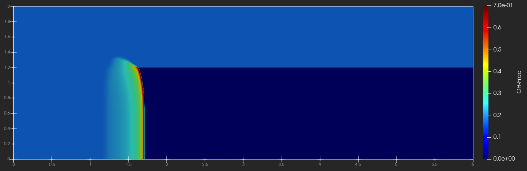
The video shows the total density ($\rho=\rho^1+\rho^2$), the density of the first ion species ($\rho^1$), and the so-called blending coefficient ($\alpha$) for the combination of a fourth-order accurate entropy stable DG method with first- and second-order accurate FV methods (Rusanov solver) and $1024^2$ degrees of freedom. A blending coefficient $\alpha=0$ means that only the DG is being used, and a blending coefficient $\alpha=1$ means that only the FV method is being used. The example shows that the hybrid FV/DG scheme is able to capture the shocks of the simulation correctly, deal with near-vacuum conditions and sharp interfaces.
[1] Rueda-Ramírez, A. M.; Pazner, W., & Gassner, G. J. (2022). Subcell limiting strategies for discontinuous Galerkin spectral element methods. Computers & Fluids. arXiv:2202.00576.
[2] Orszag, S.; Tang, C (1979). Small-scale structure of two-dimensional magnetohydrodynamic turbulence. Journal of Fluid Mechanics.
[3] Persson, P. O.; Peraire, J. (2006). Sub-cell shock capturing for discontinuous Galerkin methods. In 44th AIAA Aerospace Sciences Meeting and Exhibit (p. 112).